Fourier Analysis of Time Series

by Dr. R. L. Herman, UNC Wilmington

Friday, September 20, 2002

This is a work in progress.

Introduction

Often one is interested in determining the frequency content of signals. Signals are typically represented as time dependent functions. Real signals are continuous, or analog signals. However, through sampling the signal by gathering data, the signal does not contain high frequencies and is finite in length. The data is then discrete and the corresponding frequencies are discrete and bounded. Thus, in the process of gathering data, one seriously affects the frequency content of the signal. This is true for simple a superposition of signals with fixed frequencies. The situation becomes more complicated if the data has an overall non-constant trend or even exists in the presence of noise.

From Transforms to Series

To be completed.

Fourier Series

As described in the last section (hopefully), we have seen that by restricting our data to a time interval [0, T] for period T, and extending the data to , one generates a periodic function of infinite duration at the cost of losing data outside the fundamental range. This is not unphysical, as the data is typically taken over a finite period of time. Thus, any physical results in the analysis can be obtained be restricting the outcome to the given period.

In typical problems one seeks a representation of the signal, valid for as

where the angular frequency is given by

Note that f(t) is periodic with period P=T: Most signals have an infinite period, so we already have made a first approximation. Thus, this has restricted the physical data to [That is, by limiting t, we are forced to using discrete frequencies, or the above sum as opposed to an integral in the Fourier Transform in the last section.]

One can extract the Fourier Coefficients () using the orthogonality of the trigonometric basis. Namely, such orthogonality for a set over the interval with weight is given by the condition

For the trigonometric functions, this is given by the relations

These relations are proved in Appendix A. The coefficients are found to in Appendix B as

Discrete Series

In the previous analysis we had restricted time to the interval [0,T], leading to a Fourier series with discrete frequencies and a periodic function of time. In reality, taking data can only be done at certain frequencies, thus eliminating high frequencies. Such a restriction on the frequency will lead to a discretization of the data in time. Another way to view this is that when recording data we sample at a finite number of time steps, limiting our ability to collect data with large oscillations. Thus, we not only have discrete frequencies but we also have discrete times.

This can be captured in the following representation:

where the time, time step and trigonometric arguments are given by

and

We need to determine M and the unknown coefficients. As for the Fourier series, we rely on an orthogonality principle, but this time replacing the integral by a sum. Again we will determine the unknowns in terms of the given samples of the function f(t). The orthogonality is provided in Appendix C. If we take N samples, we can the determine N unknown coefficients and Thus, we can fix Often the coefficients and are included for symmetry. Note that the corresponding sine function factors evaluate to zero, leaving these two coefficients arbitrary. Thus, we can take them to be zero.

The full set of coefficients are found to be (in Appendix D)

Matlab Implementation

In this section we provide implementations of the discrete trigonometric transform in Matlab. The first implementation is a straightforward one which can be done in most programming languages. The second implementation makes use of matrix computations that can be performed in Matlab. Sums can be done with matrix multiplication, as describes in Appendix I. This eliminates the loops in the program.

Direct Implementation without special use of matrix algebra

% DFT in a direct implementation

% Enter Data in y

y=[7.6 7.4 8.2 9.2 10.2 11.5 12.4 13.4 13.7 11.8 10.1 ...

9.0 8.9 9.5 10.6 11.4 12.9 12.7 13.9 14.2 13.5 11.4 10.9 8.1];

% Get length of data vector or number of samples

N=length(y);

% Compute Fourier Coefficients

for p=1:N/2+1

A(p)=0;

B(p)=0;

for n=1:N

A(p)=A(p)+2/N*y(n)*cos(2*pi*(p-1)*n/N)';

B(p)=B(p)+2/N*y(n)*sin(2*pi*(p-1)*n/N)';

end

A(N/2+1)=A(N/2+1)/2;

% Reconstruct Signal - pmax is number of frequencies used in increasing order

pmax=13;

for n=1:N

ynew(n)=A(1)/2;

for p=2:pmax

ynew(n)=ynew(n)+A(p)*cos(2*pi*(p-1)*n/N)+B(p)*sin(2*pi*(p-1)*n/N);

end

% Plot Data

plot(y,'o')

% Plot reconstruction over data

hold on

plot(ynew,'r')

hold off

Compact Implementation

This implementation uses matrix products and is described in Appendix H.

% DFT in a compact implementation

% Enter Data in y

y=[7.6 7.4 8.2 9.2 10.2 11.5 12.4 13.4 13.7 11.8 10.1 ...

9.0 8.9 9.5 10.6 11.4 12.9 12.7 13.9 14.2 13.5 11.4 10.9 8.1];

N=length(y);

% Compute the matrices of trigonometric functions

p=1:N/2+1;

n=1:N;

C=cos(2*pi*n'*(p-1)/N);

S=sin(2*pi*n'*(p-1)/N);

% Compute Fourier Coefficients

A=2/N*y*C;

B=2/N*y*S

A(N/2+1)=A(N/2+1)/2;

% Reconstruct Signal - pmax is number of frequencies used in increasing order

pmax=13;

ynew=A(1)/2+C(:,2:pmax)*A(2:pmax)'+S(:,2:pmax)*B(2:pmax)';

% Plot Data

plot(y,'o')

% Plot reconstruction over data

hold on

plot(ynew,'r')

hold off

Appendices

A. Orthogonality of Trigonometric Basis

We want to prove the relations (for , )

These are based upon the trigonometric identities in Appendix F. For

since and for n and m integers. Similarly, the other integrals can be computed.

since Finally,

For we have instead

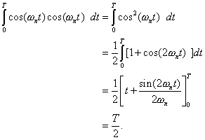
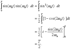
Here we have used the trigonometric identities and , which are obtainable from the identities in Appendix F.

B. Derivation of Fourier Coefficients

We now look at the Fourier series representation

We can use the orthogonality relations in the last Appendix in order to arrive at expressions for the Fourier coefficients.

First, we integrate the series over one period.

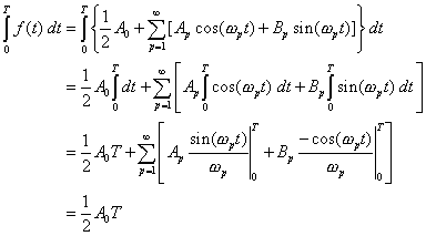
This will give the expression

Now multiply the series by for some and integrate.

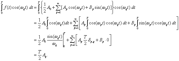
Here use was made of the known orthogonality relations from the last section. Also, the Kronecker delta was used, defined as

This renders the sum above a sum with all zero terms except for one, that for

For example, if we have

Thus, one can solve for the 's to obtain

Similarly, one has

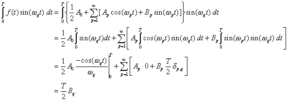So,

C. Discrete Orthogonality

The derivation of the discrete Fourier coefficients can be done using the discrete orthogonality of the discrete trigonometric basis similar to the derivation of the above Fourier coefficients for the Fourier series. We first prove the following

This can be done more easily using the exponential form,

by using Euler's formula, for each term in the sum.

The exponential sum is the sum of a geometric progression, which can be summed as done in Appendix G. Thus, we have

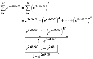
As long as the numerator is 0. In the special cases that , we have So,

Therefore,

and the result follows.

We can use this to establish orthogonality relations of the following type for :

Splitting the above sum into two sums and then evaluating the separate sums from earlier in this section,

we obtain

Similarly, we find

and

D. Discrete Transform

The derivation of the coefficients for the DFT is now easily obtained using the discrete orthogonality in the last section. We start with the expansion

We first sum over n:

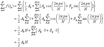
Now, we can multiply both sides of the expansion by and sum over n.

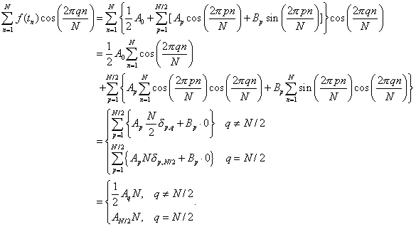So, we have found that

Similarly,

Finally, we have

E. The Discrete Exponential Transform

The derivation of the coefficients for the DFT was obtained using the discrete orthogonality in the last section. However, this is not the form used in Matlab for spectral analysis. Matlab allows for the computation of the Fast Fourier Transform (FFT) and its description in the help section does not involve sines and cosines. Namely, Matlab defines the transform and inverse transform as

"For length N input vector x, the DFT is a length N vector X, with elements

X(k) = sum x(n)*exp(-j*2*pi*(k-1)*(n-1)/N), 1 <= k <= N.

n=1

The inverse DFT (computed by IFFT) is given by

x(n) = (1/N) sum X(k)*exp( j*2*pi*(k-1)*(n-1)/N), 1 <= n <= N.

k=1

The relationship between the DFT and the Fourier coefficients a and b in

N/2

x(n) = a0 + sum a(k)*cos(2*pi*k*t(n)/(N*dt))+b(k)*sin(2*pi*k*t(n)/(N*dt))

k=1

a0 = X(1)/N, a(k) = 2*real(X(k+1))/N, b(k) = -2*imag(X(k+1))/N,

where x is a length N discrete signal sampled at times t with spacing dt."

Or, it also provides the following:

where for

In this section we will derive the discrete Fourier exponential transform in preparation for a discussion of FFT in the next section. We will start with the DFT.

Again, we can employ Euler's formula to rewrite the trigonometric functions in terms of exponentials, Namely, using we have that

Then we have

We define and note that the above result can be written as

Here we have introduce the complex conjugate operation

The terms in the sums look similar. We can actually combine them into one form. Note that Thus, we can write

in the second sum. Since , we see that So, we can rewrite the second sum as

Since q is a dummy index (it can be replaced by any letter without changing the value of the sum), we can replace it with a p and combine the terms in both sums to obtain

where

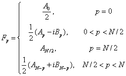
Notice that the real and imaginary parts of the Fourier coefficients obey certain symmetry properties over the full range of the indices since the real and imaginary parts are related between and [A description of this will be provided later.]

We can know determine the coefficients in terms of the sampled data.

Thus,

and

We have shown that for all F's but two, the form is

However, we can easilty show that this is also true when and

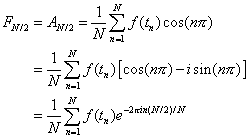
and

Thus, all of the 's are of the same form. This gives us the discrete transform pair

Note that this is similar to the definition of the FFT given in Matlab.

F. Fast Fourier Transform

The usual computation of the discrete Fourier transform is done using the Fast Fouier Transform (FFT). There are various implementations of it, but a standard form is the Radix-2 FFT. We describe this FFT in the current section. We begin by writing the DFT compactly using . Note that and We can then write

The key to the FFT is that this sum can be written as two similar sums:

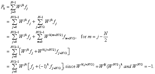
Thus, the sum appears to be of the same form as before, but there are half as many terms with a different coefficient for the 's. In fact, we can separate the terms involving the + or – sign by looking at the even and odd values of k.

For even we have

For odd we have

Each of these equations gives the Fourier coefficients in terms of a similar sum using fewer terms and with a different weight, IF N is a power of 2, then this process can be repeated over and over until one ends up with a simple sum.

The process is easily seen when written out for a small number of samples. Let Then a first pass at the above gives

The point is that the terms in these expressions can be regrouped with and noting :

However, each of the g-series can be rewritten as well, leading to

Thus, the computation of the Fourier coefficients amounts to inputting the f's and computing the g's. This takes 8 additions and 4 multiplications. Then one get the h's, which is another 8 additions and 4 multiplications. There are three stages, amounting to a total of 12 multiplications and 24 additions. Carrying out the process in general, one has steps with multiplications and N additions per step. In the direct computation one has multiplications and additions. Thus, for that would be 49 multiplications and 56 additions.

The above process is typically shown schematically in a "butterfly diagram". Examples can be found at other sites. One might be provided here at a later date. For now, we have the basic butterfly transformation displayed as

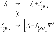
In the actual implementation, one computes with the h's in the following order:

Output and Binary Representation

Desired Order

The binary representation of the index was also listed. Notice that the output is in bit-reversed order as compared to the right side of the table which shows the coefficients in the correct order. [Just compare the columns in each set of binary representations.] So, typically there is a bit reversal routine needed to unscramble the order of the output coefficients in order to use them.

G. Trigonometric Identities

The basic trigonometric identities that one needs the product of trigonometric functions expanded as simple expressions. These are based upon the sum and difference identities:

Adding or subtracting one obtains

H. Geometric Progression

Another frequently occurring computation is the sum of a geometric progression. This is a sum of the form . This is a sum of terms in which consecutive terms have a constant ratio, The sum is easily computed. One multiplies the sum by and subtracts the resulting sum from the original sum to obtain

Factoring on both sides of this chain of equations yields the desired sum,

I. Matrix Operations for Matlab

The beauty of using Matlab is that many operations can be performed using matrix operations and that one can perform complex arithmetic. This eliminates many loops and make the coding of computations quicker. However, one needs to be able to understand the formalism. In this section we elaborate on these operations so that one can see how the Matlab implementation of the direct computation of the DFT can be carried out in compact form as shown previously in the Matlab Implementation section. This is all based upon the structure of Matlab, which is essentially a MATrix LABoratory.

A key operation between matrices is matrix multiplication. An matrix is simply a collection of numbers arranged in n rows and m columns. For example, the matrix

is a matrix. The entries (elements) of a general matrix A can be represented as which represents the ith row and jth column.

Given two matrices, A and B, we can define the multiplication of these matrices when the number of columns of A equals the number of rows of B. The product, which we represent as matrix C, is given by the ijth element of C. In particular, we let A be amatrix and B an matrix. The product, C, will be a matrix with entries

If we wanted to compute the sum , then in a typical programming language we could use a loop, such as

Sum =0
Loop n from 1 to N
Sum = Sum + a(n)*b(n)

End Loop

In Matlab we could do this with a loop as above, or we could resort to matrix multiplication. We can let a and b be and matrices, respectively. Then the product would be a matrix; namely, the sum we are seeking. However, these matrices are not always of the suggested size.

A matrix is called a row vector and a matrix is called a column vector. Often we have that both are of the same type. One can convert a row vector into a column vector, or vice versa, using the matrix operation called a transpose. More generally, the transpose of a matrix is defined as follows: has the elements satisfying .

In Matlab, the transpose if a matrix A is .

Thus, if we want to perform the above sum, we have . In particular, if both a and b are row vectors, the sum in Matlab is given by and if they are both row vectors, the sum is This notation is much easier to type.

In our computation of the DFT, we have many sums. For example, we want to compute the coefficients of the sine functions,

The sum can be computed as a matrix product. The function y only has values at times This is the sampled data. We can represent it as a vector. The sine functions take values at arguments (angles) depending upon p and n. So, we can represent the sines as an or matrix. The Fourier coefficient thus becomes a simple matrix multiplication, ignoring the prefactor . Thus, if we put the sampled data in a vector Y and put the sines in an vector S, the Fourier coefficient will be the product, which has size . Thus, in the code we see that these coefficients are computed as B=2/N*y*S for the given y and B matrices. The A coefficients are computed in the same manner. Comparing the two codes in that section, we see how much easier it is to implement. However, the number of multiplications and additions has not decreased. This is why the FFT is generally better. But, seeing the direct implementation helps one to understand what is being computed before seeking a more efficient implementation, such as the FFT.