SAMPLING SEDENTARY ORGANISMS
I. Objectives:
1. Introduce basic
approaches for sampling sedentary organisms
2. Provide experience with application of
transect and quadrat sampling
II. Introduction:
Ecologists have the challenge of evaluating the nature and function of natural systems. However, they are often faced with the problem that they cannot accurately determine many important parameters strictly through qualitative observations. Problems with spatial scale often make it difficult to directly estimate average densities in habitats such as large forested tracts or in aquatic habitats where one cannot directly see the animals or plants of interest. To measure functions in natural system, it is necessary to representatively sample both the biotic and abiotic components. Since it is usually impossible to sample an entire population within a study area, one must take smaller samples of the community or population of interest. The problem then becomes how to best estimate the parameters of some ecological system taking into account limited time and resources. The problem of sampling can be thought of as several issues: 1) what sampling method can be used to collect the needed data, 2) how do we select sampling locations to limit potential bias and obtain best estimates of target parameters, and 3) how can we minimize the number of samples we take while still providing an accurate estimate of parameters?
Ecologists have developed several basic sampling approaches to deal with sedentary (non-moving) organisms. The most common method is plot sampling. This method is relatively straightforward in that it simply involves counting the number of organisms of interest in a defined area (often, but not necessarily, a quadrat). Plot sampling is a highly versatile approach, providing information on densities, associations, dispersion patterns, and indirect evidence on a variety of community or population processes. However, three problems with this method that will be explored in this lab are the size of the sampling plot, how plots will be placed, and the number of plots to be sampled. The size of the plot must obviously vary with the size of the organisms to be sampled, but also may need to be varied depending on distributions of organisms or the size of habitat patches in the environment. It is often useful to have a plot smaller than the average patch size to get information of dispersion patterns, mean numbers within patches, and densities between patches. Also, larger plots tend to give more accurate estimates of overall densities, but are more cumbersome and time consuming to place and sample. The placement of plots needs to be done so that there is no bias in the data collected. This is usually achieved through random or haphazard placement (what is the difference?), but may also be limited by time and resources.
When organisms are known to vary across some defined gradient, a variation of the plot sampling method that is often used is a belt transect. This involves sampling replicate rectangular belts that straddle a known environmental gradient. Often these belts are broken into subsections. The problems of size (and shape), placement, and number of replicates also apply to belt transects.
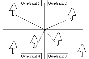
An alternative to plot sampling methods are a variety of methods collectively known as plotless sampling approaches. These approaches are generally quicker to apply than plot sampling, but usually provide much more limited information. The most common plotless sampling method is point-quarter sampling. Point-quarter sampling can provide density measures if applied correctly and has the advantage over plot sampling that it is less cumbersome and time-consuming than sampling of larger quadrats. However, it has the disadvantages that density estimates may not be accurate if organisms have severely clumped or uniform distributions and the technique does not provide as versatile information as obtained with quadrat sampling. The basic methodology for point-quarter sampling is: 1) randomly (or haphazardly) select a center point, 2) divide the area around the center point into 4 quadrants (pie sections), with the quadrants crossing at the center point, and 3) record the distance to the nearest tree (or species of interest) in each quadrant.

This procedure is then repeated for additional replicates. Density of trees for Point-quarter sampling can be determined with the following formula:
D=1/A and A=(Edi/PQ)2
Where:
D=density in distance units squared A=area occupied by trees
di=distance from the center point to the nearest tree in the ith quadrant
P=number of center points
Q=number of quadrants taken for each center point (usually 4)
PQ=number of center points times the number of quadrants per point
Another method used to obtain qualitative information on the distribution and abundance of sedentary organisms is the line transect. This method simply involves placing a line of pre-determined length over an area and then recording the number of organisms intercepted by that line (or within a defined distance of the line). This method has the advantage of being quick and easy, but has the disadvantage of providing information on only relative abundances and not giving quantitative information on actual densities.
III. Methodology - Computer Sampling Simulation.
We will use the Ecobeaker program to investigate several aspects of quadrat sampling, especially how size, number and shape of quadrats taken affect accuracy of quadrat results.
A. The Ecobeaker Universe
The Ecobeaker universe presents a 50m X 50m landscape with 3 different types of plants on it, each a different color. The green plants are growing in completely random places around the landscape. The blue plants grow much better when they are near other blue plants, so they are clumped together (a patchy distribution). The red plants compete strongly with each other, so they do not like to grow nearby other red plants. This makes the red plants space themselves out in a somewhat even pattern. There are exactly 80 individuals of each plant type in the whole area.
B. Getting into the program
1. Double click on the
Ecobeaker icon
2. Open the file "Random Sampling"
using the open command in the file menu.
3. When it is open, you should get a screen
that shows the landscape to be sampled in the
upper left
of the screen. To the right of the landscape are the Species and
Population size windows,
which show the
color and total number for each species. The Sampling parameters
window lets you
change the width, height and number of quadrats which you use to
sample the populations.
The Control
panel window lets you actually take a sample (by clicking on
"sample").
C. Effect of size, keeping replication constant
1. The program has an
initial, default quadrat size of 5m x 5m.
2. Click on the sample button in the
Control panel to take a sample. A square will be drawn on
the
Landscape window, showing the area that is being sampled. Just
below the Landscape
window a dialog box will appear, telling you how many individuals
of each species were found
within this square. Write down both the number of individuals of
each species and the width
and
height of the area sampled.
3. Repeat this procedure at least 4 more
times (5 total), so that you get a range of different
estimates
that tell you whether you can expect this scheme to consistently
give you accurate
and
precise results.
4. Now increase the size of the
sampling quadrat to a larger size such as 10m x 10m. To do this,
go
to the Sampling parameters window and type "10" for
both the quadrat height and quadrat
width
items. Then click on the change button in the sampling parameters
window to make the
change
in size you specified go into effect.
5. Repeat the sampling procedure
for the larger quadrat size.
6. Repeat the entire procedure for
at least two more quadrat sizes (e.g. 15m x 15m, 20m x
20m).
7. When you have finished your
sequence, estimate the true population size (number in the entire
50m
x 50m landscape) from each sample you took for each species.
Present the results in a
table
form. Next, make a plot of population estimate (y-axis) versus
quadrat area (x-axis) for
each
species. This will show you visually what happened to your
estimate as you increased
quadrat
size. You will have several pionts plotted for each quadrat size,
from each of the
samples
you took at that size, and this will show you the range of
accuracy you might expect
from
a quadrat of that size.
8. What are the shapes of your estimated
population size versus quadrat area graphs for each
species?
Is there some point where increasing the size of the quadrat
seems to make little
difference
in accuracy? Is this point the same for all the species?
D. Effects of quadrat shape
1. Change your quadrat size to 10m x
10m and do sampling as described above.
2. Repeat this procedure with 3 other plot
shapes that have the same area (e.g., 5m X 20m, 4m
X 25m, 2m x
50m).
3. Estimate the true population sizes and
construct graphs as described in #7 above (in this
case, the
y-axis would be estimated population size and the x-axis would be
quadrat shape ordered
from most
narrow shape to exact square).
4. How did changing quadrat shape affect
population estimates? Is the affect the same for
all
species?
E. Influence of replicate sampling
1. Set the quadrat size
back to 5m x 5m and take 5 sets of samples as described above.
2. Now go to the Sampling
parameters window and change the number of quadrats
to 2. This
time,
when you take a sample, first one 5m x 5m quadrat will appear, as
before, and a dialog
box
will tell you how many individuals of each species were found in
that quadrat. When you
click
on the continue button, a second 5m x 5m quadrat will be laid
down, and again you’ll
receive
a report of how many individuals were found in the second
quadrat. Finally, a third
dialog
box will appear giving you the total number of individuals found
within both quadrats.
For
the purposes of this lab, you should calculate the mean number
per quadrat (total number
divided
by number of replicate quadrats per sample). Repeat this sampling
procedure 5 times
(5
pairs of quadrats).
3. Repeat the sampling procedure
described in step 2 of this section for 5 replicates and 7
replicates
per sampling period, recording means for each.
4. Estimate the true population
sizes and construct graphs as described in #7 above (under
quadrat
size). The x-axis in this case will be number of replicate
quadrats used and the y-axis
will
be population estimates for each sampling set.
5. Do these graphs look the same
as those you got with a single quadrat? Does accuracy of your
estimate
change with increasing replication?
IV. Laboratory Assignment
Turn in graphs and answers to questions in sections
C8, D4 and E5.
V. Key Points From The Homework:
1. As you increase the plot size,
accuracy increases but the sampling becomes
more cumbersome and
time-consuming.
You
may use the smallest plot sizes for species that are distributed
evenly; you need to
use larger plot sizes for species that are clumped.
2. When sampling a clumped species, it is best to use belt
transects.
3. As you increasing the number of replicates, accuracy increases
but the sampling also becomes
more cumbersome.
Return to Ecology Lab Syllabus