PSY 555 Homework 15
Answers
Chapter 9: #9,12,17,23,24,25
9.9(a). Cerebral hemorrhage in low-birthweight
infants and cognitive deficit at age 5:
Power
calculation:
d=.20
N=25 r=.20
![]()
Power=.17
The
power of the test is approximately .17.
9.9(b). Power of .80![]() r=.20
r=.20
2.80=.20![]()
![]()
![]()
197
infants would be required to have a power of .80.
9.12.


![]()

![]()
![]()
The
95% confidence limits on b* are -.0019 and .1397.
9.17.


![]()
![]()
![]()

For
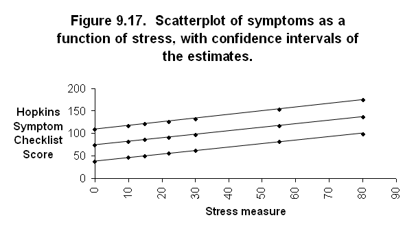
several different values of X (i.e., 0,10,15,22,30,55,80), calculate the
corresponding predicted values of Y and s'Y.X and plot the
results.
Y(30)=97.453
Y(22)=91.1882
Y(15)=85.7065
Y(10)=81.791
Y(80)=136.539
Y(0)=73.891
Y(55)=117.0305

s'Y.X(30)=17.632
s'Y.X(22)=17.597
s'Y.X(15)=17.617
s'Y.X(10)=17.66
s'Y.X(80)=19.169
s'Y.X(0)=17.816
s'Y.X(55)=18.128
CI
Y(30)=62.471 to 132.435
CI
Y(22)=56.276 to 126.100
CI
Y(15)=50.754 to 120.659
CI
Y(10)=46.754 to 116.828
CI
Y(80)=98.508 to 174.570
CI
Y(0)=38.544 to 109.238
CI
Y(55)=81.065 to 152.996

9.23(a). r1=.68 N=17 ![]()
r2=.53
N=28
![]()

z=.716![]() not significant, p=.4716
not significant, p=.4716
The
relations were not significantly different, z=.716,
p=.4716.
9.23(b). There
is no support, based on this data, for the hypothesis that reading the passage
affects the relation between SAT verbal score and the 100-item test
performance.
9.24. r1=.88 N=52 ![]()
![]()
r2=.72
N=74 ![]()
![]()

These
correlations are significantly different, z=2.52,
p<.0018.
9.25. The
significance achieved by the second set of correlations is probably due to the
larger N values (74 and 52), although it could possibly be due to the fact that
the correlations originally were higher in the second problem (so these values are
more likely to differ b/c smaller differences will be significant). The higher sample sizes, however, are most
likely responsible for the difference in terms of significant findings between
the two problems.
1. When you restrict the range of the data
points you examine, the correlation may be altered from what it would have been
if the range was not restricted. The
altered correlation may be either larger or smaller than t unrestricted range
correlation, although generally the altered correlation will be smaller. An example would be standardized test scores
(e.g., SAT, GRE) that are used to predict college performance. While the relation between such measures is
assumed to be high, the correlations are generally moderate in size (e.x.,
r=.65). This lower correlation (at least
lower than would be expected) is due to the fact that only a portion of the
people who take these tests get into college (generally, the people with better
scores). So, the correlation between SAT
and college performance, as measured by GPA, is based on a restricted range of
data and is, in all likelihood, smaller than the correlation that would be
obtained if all people who took the SAT went to college and all this data was
examined.
Heterogeneous subsamples pose a problem for
correlations. For example, many
relations between variables can be obscured by the presence of a third variable
(e.g., gender). Many relations are not
obvious when both genders are examined.
However, when genders are examined separately, these relations are
evident. So, anytime data is collected
from separate groups (or data sources), researchers should be cautious when
examining relations for the aggregate data.
It probably would be more prudent to examine the desired relation for
each group separately.
2(a). r=.53
r=.42
H0=There
is no significant difference between correlations obtained in the two studies (r1=r2).
H1=There
is a significant difference between the correlations obtained in the two
studies (r1![]() r2).
r2).
2(b). The
correlation found in the first study (r=.53) is significantly greater
than the correlation found in subsequent study (r=.42), z=2.5, p<.0124.